Determine Weights Of Evidence Ranges
Description
This container defines the best ranges or intervals employed to categorize continuous gray-tone variables.
Inputs
| Name | Type | Description |
|---|---|---|
| Initial Landscape | Categorical Map Type | Initial map of land use and cover classes. |
| Final Landscape | Categorical Map Type | Final map of land use and cover classes. |
| Skeleton | Weights Of Evidence Skeleton Type | Spatial variables selected and their types - Category or continuous gray-tone -, and the parameters specified for range definitions, such as increment, maximum and minimum deltas, and tolerance angle. |
Optional Inputs
| Name | Type | Description | Default Value |
|---|---|---|---|
| Fix Abnormal Weights | Boolean Value Type | If true, recalculate abnormal weights. Otherwise, assume abnormal values are zero. | False |
Outputs
| Name | Type | Description |
|---|---|---|
| Ranges | Weights Type | Intervals defined for continuous gray-tone variable. |
Group
Notes
The Weights of Evidence calculations, which employ binary patterns, can be extended to multiple category maps, by treating in each case one category versus all other categories combined, whose areas are added to represent (). Agterberg & BonhamCarter (1990) also present an extension of this method to gray-tone maps (e.g., a map of distances to road), by defining intervals for these maps.
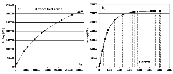
A key issue to any categorization process concerns the preservation of the data structure. The present method adapted from Agterberg & BonhamCarter (1990), calculates ranges according to the data structure by first establishing a minimum delta (Dx) for a continuous gray-tone variable x that is used to build n incremental buffers (Nx) comprising intervals from xminimum to xminimum + nDx. Each n defines a threshold that divides the map into two classes: (Nx) and (). An is the number of cells for a buffer (Nx) multiple of n and dn is the number of occurrences for the modeled event (D) within this buffer. The quantities An and dn are obtained for an ordered sequence of buffers N(xminimum + nDx). Subsequently, values of W+, C, and S2 for each buffer are calculated using equations 2 to 8.
A sequence of quantities An is plotted against . Thereafter breaking points for this graph are determined by applying a line-generalizing algorithm (Intergraph, 1991) that contains three parameters:
- minimum distance interval along x, mindx,
- maximum distance interval along x, maxdx, and
- tolerance angle ft.
For dx (a distance between two points along x) greater than mindx or lesser than maxdx, a new breaking point is placed whenever dx > maxdx or f (an angle between v and v’ - vectors linking the current to the last point and the last point to its antecedent, respectively) exceeds the tolerance angle ft. Thus, the number of ranges decreases as a function of ft. The ranges are finally defined by linking the breaking points with straight lines. Note that An is practically error-free whereas dn is subject to a considerable amount of uncertainty because it is regarded as the realization of a random variable. Since small An can generate noisy values for W+, Goodacre et al. (1993) suggest that, instead of calculating by employing equations 2 and 4, one should estimate W+ for each defined range through the following expression:
(10)
where and k represents the breakpoints defined for the n increments of Dx.

In sum, the application of Weights of Evidence in a change analysis aims at selecting the most important variables as well as quantifying their influences on each type of transition. Weights of evidence are assigned for each range or category of a variable represented by its cartographic layer and a post-probability map is obtained from the integration of these weights of evidence. This map points out the most favorable areas for a transition, thus it can be interpreted as a map of spatial transition probability. As a result, this empirical relationship, determined by Weights of Evidence, can be used to parameterize and calibrate spatial simulation models such as Dinamica EGO. Although Weights of Evidence can be classified as a local operator, because it only computes values from overlapping map locations (x,y), the use of chorographic variables, like distance to a geographic feature, ensures the capture of the neighborhood effect in this calculation.
References
Agterberg, F.P. and Bonham-Carter, G.F., 1990: Deriving weights of evidence from geoscience contour maps for the prediction of discrete events. XXII Int. Symposium AP-COM, 381-395.
Intergraph Corporation, 1991. Intergraph Microstation PC, Version 4 User’s Guide. Bentley Systems, Inc. and Intergraph Corporation, 333 pp.
Internal Name
DetermineWeightsOfEvidenceRanges