We evaluated several map comparison methods, and found that Reciprocal Similarity Comparison dealt best with comparison of changes.
Introduction
Uncertainty in modeling can originate from several sources, including incomplete knowledge of human-natural systems, misconception about the main system processes, lack of data, structural limits of the model itself, the impossibility of finding an optimal set of parameters able to cover multiple space-time resolutions and spans, level of stochasticity, and/or an incomplete statistical/heuristic learning process (Pontius Jr. and Spencer, 2005; Messina et al., 2008; Pontius and Neeti, 2010; Pontius Jr. and Petrova, 2010).
The terms verification and validation have often been confused and used interchangeably (Oreskes et al., 1994; Rykiel, 1996). Verification checks the ability of a model to meet the needs of the final user and attempts to identify internal logical/computational errors, while validation measures a model’s ability to represent cause-effect relations in site-specific contexts (Coquillard and Hill, 1997).
Validation refers to the comparison between model predictions and observations stored in the dataset that were not used to train the model. Thus, during validation the calibrated model is fed with new values, independent from the training dataset. Training and validation datasets are commonly created by randomly splitting observational data into two sub-sets, e.g. 80% of data for training and 20% for validation (Chung and Fabbri, 2003; Villa-Vialaneix et al., 2012), or by using time partitioning (i.e. calibration employs older records or time span, while validation uses the most recent records or time span (Pontius Jr. and Petrova, 2010).
Choosing the best goodness-of-fit criterion for validation depends strictly on data type and quality, project goals, and required accuracy. Even if model output is consistent with the training and test datasets, there is no guarantee that the model will perform equally well when tested with a different dataset for predictive purposes. For example, information captured by historical data could contain errors (Pontius Jr. and Petrova, 2010), or may be outdated and thus unrepresentative of present and future system dynamics. Alternatively, a paucity of data may require selection of calibration and validation time intervals much shorter than the future period the model aims to predict (Pontius and Neeti, 2010). Finally, uncertainty surrounds whether the employed validation method is truly measuring model accuracy (Hagen-Zankera and Lajoie, 2008).
Spatial models require comparison within a neighborhood context, because maps that do not match exactly cell-by-cell may still present similar spatial patterns and therefore spatial agreement within a given cell vicinity. To address this issue, several vicinity-based comparison methods have been developed. For example, Costanza (1989) introduced the multiple-resolution fitting procedure that compares map spatial fitness within increasing window sizes. Power et al. (2001) provided the Fuzzy Inference System, a method based on hierarchical fuzzy pattern matching. Pontius Jr. (2000, 2002) introduced Klocation, which differentiates errors due to location and quantity. Hagen et al. (2003) developed the Kfuzzy, considered equivalent to the Kappa statistic, and the Fuzzy Similarity, which accounts for fuzziness of location and category within a cell neighborhood. Almeida et al. (2008) modified the latter and named it Reciprocal Similarity Comparison, because this metric corresponds to the minimum fuzzy similarity between map 1 of changes versus map 2 of changes and vice versa (Soares-Filho et al. 2009), (Fig. 1). Van Vliet et al. (2011) developed the Kappa Simulation, which assesses the agreement between the simulated land-use map and the actual one, based on the original land-use map.
We evaluated six map comparison methods using a set of synthetic maps (Fig. 2). The best methods are the ones that yield the highest contrast between the reference map (Final) and a randomly blurred pattern (neutral model), but also capture similitude between maps that closely resemble each others, such as the maps of line1 x line2 (table 1). The best method is the Reciprocal Similarity Comparison, with exponential decay function truncated at 19×19-window size. This method was chosen because it focuses only on the goodness-of-fit of the changes rather than the whole map, clearly distinguishes well-matched spatial patterns from a neutral model (a random map with same number of changes; probability for all cells =0.5), and is virtually independent of window size of comparison if large windows are employed.

Fig. 1 – Diagram of the deforestation model together with its fitness evaluation function in the Dinamica EGO graphical interface. The sets of functors within the two outer Group functors are represented in Fig. 1 of the main text as being embedded in “model” and in “fitness function”. 1) calculates the period transition matrix, 2) integrates the Weights of Evidence coefficients previously calculated to produce the transition probability map, 3) transforms the net rates into number of cells to change, 4) spatially allocates the changes (in this case, the model only used the Patcher functor that was set to not form patches), 5) calculates the historical and 6) simulated map of changes, and 7) evaluates Reciprocal Fuzzy Similarity between historical and simulated maps and 8) finds the minimum.
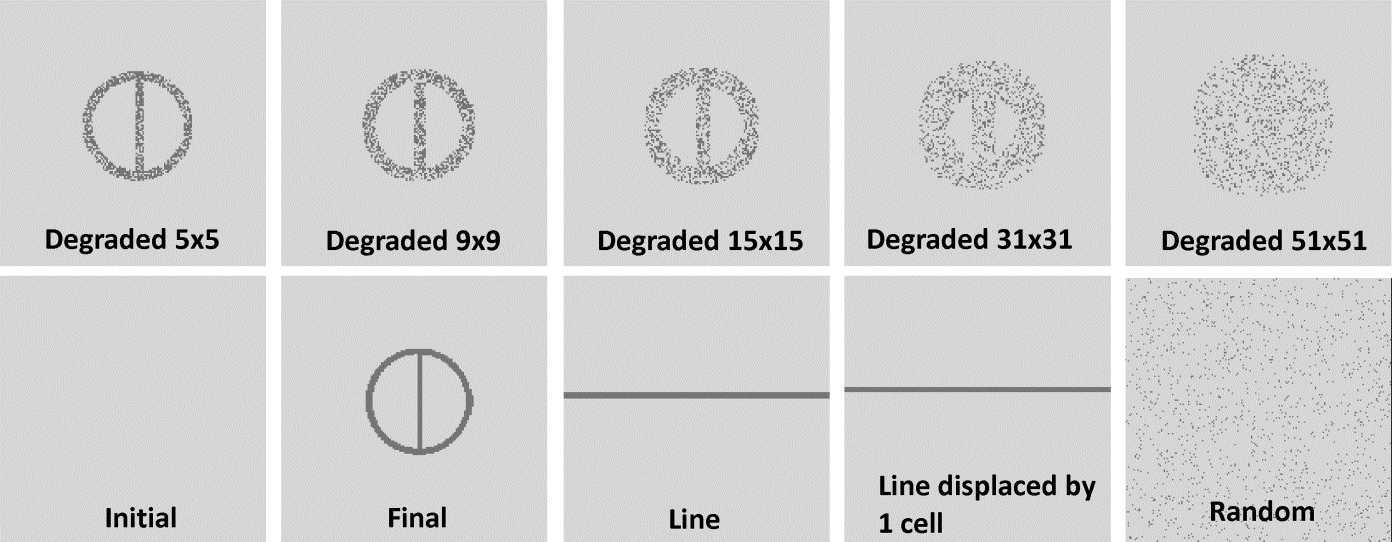
Fig. 2 – Set of maps used to evaluate map comparison methods. All maps are derived from “Initial” using the same number of changes from “Initial” to “Final”. Reference maps are “Final” and “Line”. “Degraded nxn” refers to the filter window size used as a probability map whose cell values equal to 0.5 inside and 0 outside the window, so that the simulation will produce a blurred version of the reference map. “Random” refers to a neutral model (Hagen-Zankera and Lajoie, 2008) with the same number of changes from “Initial” to “Final” allocated using a probability map with all cell values = 0.5.
| Authors | Almeida et al. (2008) Reciprocal Similarity | Power et al. (2001) | Hagen (2003) | Van Vliet et al. (2011) | Pontius Jr. (2000) | Constanza (1989) | ||
| Method \ Map Comparison | 3x3 Const | 5x5 Const | 19x19 Exp | Fuzzy Inference System | Fuzzy Kappa | Kappa Simulation | KLocation | Multiple Resolution Procedure |
| Final x Final | 100% | 100% | 100% | 84% | 100% | 100% | 100% | 100% |
| Final x Degraded 5x5 | 83% | 100% | 86% | 83% | 70% | 66% | 65% | 98% |
| Final x Degraded 9x9 | 62% | 75% | 71% | 82% | 47% | 48% | 48% | 97% |
| Final x Degraded 15x15 | 46% | 55% | 54% | 81% | 24% | 34% | 34% | 96% |
| Final x Degraded 31x31 | 26% | 32% | 32% | 80% | -3% | 18% | 18% | 95% |
| Final x Degraded 51x51 | 19% | 23% | 23% | 80% | -13% | 12% | 12% | 95% |
| Final x Random | 4% | 5% | 5% | 79% | -42% | -2% | 0% | 90% |
| Line1 x Line2 (Line x Line Displaced by 1 Cell) | 100% | 100% | 71% | 81% | 59% | -2% | -2% | 99% |
Table 1 – The method of Almeida et al. (2008) was calculated using Dinamica EGO. We implemented the method of Costanza (1989) and used 3×3 window size. We ran the method of Pontius Jr. (2000) using the version available on IDRISI 32.2 and the other metrics using the Map Comparison Kit 3.2.. For Reciprocal Similarity metrics, 3×3 and 5×5 refer to window sizes and const. to a constant function in which a value 1 is assigned if a match is found and 0 if not found within the comparison window; 19×19 exp. refers to an exponential decay function truncated at 19×19 window size (Beyond this threshold there is no significant change in this metric). Fuzzy Inference System was calculated with the option “symmetric by taking the average”. Fuzzy Kappa was calculated using exponential decay with 4×4 radius, having distance=2, slope=0.5, value=0.5. Map “initial” from Fig. 1 is used as original map in Kappa Simulation.
Conclusion
Most comparison metrics are not mutually comparable, nor are the scores of a specific metric comparable when applied to different models, given their different contexts (Hagen-Zankera and Lajoie, 2008). Our selected metric intrinsically incorporates a neutral model of permanence and can be used against a neutral model of random allocation to test whether the model predicts better than chance. Yet, benchmark for accepting or rejecting a model remains an open question.
Caution
Spatial performance is not everything. Top performance will make the model, in a deterministic way, concentrate simulated changes only on cells with high spatial transition probabilities. Hence, increased model performance, in terms of strictly spatial accuracy, may decrease model realism because land-use changes include a stochastic component. Therefore, probabilistic models should also attempt to replicate the probability distribution function of actual changes. Furthermore, land-use change models need to replicate landscape structure. This is particularly important for high spatial resolution models that aim to simulate the statistical distribution of patch sizes and forms of change, which may be multimodal due to the presence of different agents of change. Adding spatial structure to changes also decreases spatial accuracy because the allocation process becomes more constrained (Soares-Filho et al., 2002).
References
Almeida, C., Gleriani, J., Castejon, E., Soares-Filho, B., 2008. Neural networks and cellular automata for modeling intra-urban land use dynamics. International Journal of Geographical Information Science 22, 943–963.
Chung, C., Fabbri, A., 2003. Validation of spatial prediction models for landslide hazard mapping. Natural Hazards 30, 451–472.
Coquillard, P., Hill, D., 1997. Modelisation et simulation d’ ecosystemes. Des modeles deterministes aux simulations par evenements discrets. ed Masson, Paris.Costanza, R., 1989. Model goodness of fit: a multiple resolution procedure. Ecological Modelling 47, 199–215.
Costanza, R., 1989. Model goodness of fit: a multiple resolution procedure. Ecological Modelling 47, 199–215.
Hagen, A., 2003. Fuzzy set approach to assessing similarity of categorical maps. International Journal of Geographical Information Science 17, 235– 249.
Hagen-Zankera, A., Lajoie, G., 2008. Neutral models of landscape change as benchmarks in the assessment of model performance. Landscape and Urban Planning 86, 284–296.
Messina, J., Evans, T., Mason, S., A.M., S., Deadman, P., Verburg, P.H., 2008. Complex systems models and the management of error and uncertainty. Journal of Land Use Science 3, 11–25.
Oreskes, N., Shrader-Frechette, K., Belitz, K., 1994. Verification, validation, and confirmation of numerical models in the earth sciences. Science 263, 641–646.
Pontius Jr., R.G., 2002. Statistical methods to partition effects of quantity and location during comparison of categorical maps at multiple resolutions. Photogrammetric Engineering and Remote Sensing 68, 1041–1049.
Pontius Jr., R.G., Neeti, N., 2010. Uncertainty in the difference between maps of future land change scenarios. Sustainability Science 5, 39–50.
Pontius Jr., R.G., Petrova, S., 2010. Assessing a predictive model of land change using uncertain data. Environmental Modelling & Software 25, 299–309.
Pontius Jr., R.G., Spencer, J., 2005. Uncertainty in extrapolations of predictive land change models. Enviroment and Planning B 32, 211–230.
Power, C., Simms, A., White, R., 2001. Hierarchical fuzzy pattern matching for the regional comparison of land use maps. International Journal of Geographical Information Science 15, 77–100.
Rykiel, E., 1996. Testing ecological models: the meaning of validation. Ecological Modelling 90, 229–244.
Van Vliet, J., Bregt, A., Hagen-Zanker, A., 2011 Revisiting Kappa to account for change in the accuracy assessment of land-use change models. Ecological Modeling 222, 1367-1375.
Villa-Vialaneix, N., Follador, M., Ratto, M., Leip, A., 2012. Metamodels comparison for the simulation of N2O fluxes and N leaching from corn crops. Environmental Modelling & Software 34, 51–66.